问题描述

现有一个较为复杂的函数接受3个参数返回一个数，希望用神经网络拟合该函数

该复杂函数暂定为

python
def fun(x1,x2,x3):
    # return x1+x2+x3+random.random()*0.1
    return (np.sin(x1) * np.cos(x2) + np.log1p(x3**2))*10 + np.random.normal(0, 0.1)

应该足够复杂了，写入data.csv备用

csv
x1,x2,x3,y
8.444218515250482,7.579544029403024,4.20571580830845,31.49327078172624
2.5891675029296337,5.112747213686085,4.049341374504143,30.589961578798203
7.837985890347726,3.0331272607892745,4.765969541523559,21.840855541786173
5.833820394550312,9.081128851953352,5.046868558173903,36.719751437665835
2.8183784439970383,7.558042041572239,6.183689966753317,37.651338224836
2.5050634136244057,9.097462559682402,9.827854760376532,40.34142256836198
...

模型构建

构建一个8层的网络，第一层有三个神经元，分别接受三个输入，最后一层有一个神经元，用于输出。中间6层为隐藏层，每层有128个神经元

python
import torch
import torch.nn as nn
class SimpleNN(nn.Module):
    def __init__(self):
        super(SimpleNN, self).__init__()
        self.fc1 = nn.Linear(3, 128)
        self.fc2 = nn.Linear(128, 128)
        self.fc3 = nn.Linear(128, 128)
        self.fc4 = nn.Linear(128, 128)
        self.fc5 = nn.Linear(128, 128)
        self.fc6 = nn.Linear(128, 128)
        self.fc7 = nn.Linear(128, 1)
        
        self.dropout = nn.Dropout(0.5)  # Dropout with 50% probability
        self.leaky_relu = nn.LeakyReLU(0.01)  # Leaky ReLU with negative slope of 0.01

    def forward(self, x):
        x = self.leaky_relu(self.fc1(x))
        x = self.dropout(x)  # Apply dropout
        x = self.leaky_relu(self.fc2(x))
        x = self.dropout(x)  # Apply dropout
        x = self.leaky_relu(self.fc3(x))
        x = self.dropout(x)  # Apply dropout
        x = self.leaky_relu(self.fc4(x))
        x = self.dropout(x)
        x = self.leaky_relu(self.fc5(x))
        x = self.dropout(x)
        x = self.leaky_relu(self.fc6(x))
        x = self.fc7(x)
        return x

模型训练

导入所需要的库

python
import pandas as pd  # 导入 pandas 库，用于数据处理
import numpy as np  # 导入 numpy 库，用于数值计算
import torch  # 导入 PyTorch 库，用于构建和训练深度学习模型
import torch.nn as nn  # 导入 PyTorch 的神经网络模块
import torch.optim as optim  # 导入 PyTorch 的优化模块
from sklearn.model_selection import train_test_split  # 导入 sklearn 的数据集划分模块
from sklearn.preprocessing import StandardScaler  # 导入 sklearn 的标准化模块
import matplotlib.pyplot as plt  # 导入 matplotlib 库，用于绘图

设置pytorch使用cuda

python
# 检查是否有可用的 GPU
device = torch.device('cuda' if torch.cuda.is_available() else 'cpu')  # 如果有 GPU 可用则使用 GPU，否则使用 CPU
print(f'Using device: {device}')  # 打印使用的设备

加载数据

从前面的data.csv中读取数据用于训练，数据应被划分为训练集和测试集

python
# 1. 加载和准备数据
data = pd.read_csv('data.csv')  # 读取 CSV 文件中的数据

X = data.iloc[:, :-1].values  # 取出数据的前几列作为特征
y = data.iloc[:, -1].values   # 取出数据的最后一列作为标签

# 将数据集划分为训练集和测试集，测试集占总数据的 20%
X_train, X_test, y_train, y_test = train_test_split(X, y, test_size=0.2, random_state=42)

训练数据应该被标准化，这样训练的效果比较好。标准化的均值和方差应该保存到模型中，便与预测时使用

python
scaler = StandardScaler()  # 初始化标准化对象
X_train = scaler.fit_transform(X_train)  # 对训练特征数据进行标准化
X_test = scaler.transform(X_test)  # 对测试特征数据进行标准化

scaler_params = {
    'mean': scaler.mean_.tolist(),
    'scale': scaler.scale_.tolist()
}

y_mean = y_train.mean()
y_std = y_train.std()

y_params = {
    'mean': y_mean,
    'std': y_std
}

读出的数组应该从内存中转移到显存中，才能使用cuda加速计算

python
# 将 numpy 数组转换为 PyTorch 的张量，并将其移动到指定的设备（CPU 或 GPU）
X_train = torch.tensor(X_train, dtype=torch.float32).to(device)
X_test = torch.tensor(X_test, dtype=torch.float32).to(device)
y_train = torch.tensor(y_train, dtype=torch.float32).view(-1, 1).to(device)  # 将标签数据转换为二维张量
y_test = torch.tensor(y_test, dtype=torch.float32).view(-1, 1).to(device)  # 将标签数据转换为二维张量

导入模型

python
# 2. 定义模型
from model import SimpleNN  # 从 model 模块导入 SimpleNN 类
model = SimpleNN().to(device)  # 实例化模型，并将模型移动到指定的设备

损失函数和优化器

python
# 3. 定义损失函数和优化器
criterion = nn.SmoothL1Loss()  # 定义均方误差损失函数
optimizer = optim.Adam(model.parameters(), lr=0.001)  # 定义 Adam 优化器，学习率为 0.001

训练模型

模型的训练分为轮次和批量，每一轮从总数据中取出一个批次的数据进行训练

python
# 4. 训练模型
num_epochs = 10000  # 训练轮数
batch_size = 30000  # 批量大小
losses = []  # 用于记录每个 epoch 的损失

for epoch in range(num_epochs):  # 遍历每个 epoch
    permutation = torch.randperm(X_train.size()[0])  # 生成一个随机排列的索引，用于打乱训练数据
    
    epoch_loss = 0  # 初始化当前 epoch 的总损失
    for i in range(0, X_train.size()[0], batch_size):  # 遍历每个批量
        optimizer.zero_grad()  # 清零梯度
        
        indices = permutation[i:i + batch_size]  # 获取当前批量的索引
        batch_x, batch_y = X_train[indices], y_train[indices]  # 根据索引获取当前批量的数据和标签
        
        outputs = model(batch_x)  # 前向传播，计算模型输出
        loss = criterion(outputs, batch_y)  # 计算损失
        
        loss.backward()  # 反向传播，计算梯度
        optimizer.step()  # 更新模型参数
        
        epoch_loss += loss.item()  # 累加当前批量的损失到 epoch 总损失中
    
    losses.append(epoch_loss)  # 记录当前 epoch 的总损失
    
    if (epoch + 1) % 100 == 0:  # 每 100 个 epoch 打印一次损失
        #计算最近100次的平均损失
        recent_losses = losses[-100:]
        recent_loss = sum(recent_losses) / len(recent_losses)
        print(f'Epoch [{epoch+1}/{num_epochs}], Loss: {recent_loss:.4f}')

然后保存模型

python
torch.save({
    'model_state_dict': model.state_dict(),
    'scaler_params': scaler_params,
    'y_params': y_params
}, 'model_with_scaler.pth')
print('模型已保存')  # 打印模型保存信息

评估模型

python
# 5. 评估模型
model.eval()  # 切换到评估模式（禁用 Dropout 和 BatchNorm）
with torch.no_grad():  # 禁用梯度计算
    predictions = model(X_test)  # 使用测试数据进行预测
    test_loss = criterion(predictions, y_test)  # 计算测试损失
    print(f'Test Loss: {test_loss.item():.4f}')  # 打印测试损失

# 6. 可视化训练过程（可选）
plt.plot(range(num_epochs), losses)  # 绘制训练损失曲线
plt.xlabel('Epoch')  # x 轴标签
plt.ylabel('Loss')  # y 轴标签
plt.title('Training Loss')  # 图表标题
plt.show()  # 显示图表

使用模型进行预测

首先应该加载模型文件，同时读取标准化参数

python
model = SimpleNN()  # 重新创建模型实例
# model.load_state_dict(torch.load('model.pth'))
# model.eval()  # 切换到评估模式
# print('模型已加载')

# 加载模型和标准化参数
checkpoint = torch.load('model_with_scaler.pth')

model.load_state_dict(checkpoint['model_state_dict'])
scaler_params = checkpoint['scaler_params']
y_params = checkpoint['y_params']

mean = torch.tensor(scaler_params['mean'], dtype=torch.float32)
scale = torch.tensor(scaler_params['scale'], dtype=torch.float32)

y_mean = torch.tensor(y_params['mean'], dtype=torch.float32)
y_std = torch.tensor(y_params['std'], dtype=torch.float32)

print('模型已加载')
print('y_mean:', y_mean)
print('y_std:', y_std)
print('mean:', mean)
print('scale:', scale)

可以使用data.csv中的数据（即训练数据）评估模型效果

python
with torch.no_grad():
    #读取data.csv
    import pandas as pd
    data = pd.read_csv('data.csv')
    #最后一列为真实数据
    y_test = data.iloc[:, -1].values
    #前面的列为特征
    X_test = data.iloc[:, :-1].values
    # 将数据转换为张量
    X_test = torch.tensor(X_test, dtype=torch.float32)
    # 使用保存的参数标准化测试数据
    X_test = (X_test - mean) / scale
    predictions = model(X_test)
    # 反标准化预测结果
    # predictions = predictions * y_std + y_mean
    #保存结果到csv
    result = pd.DataFrame(columns=['predictions', 'y_test'])
    result['predictions'] = predictions.view(-1).numpy()
    result['y_test'] = y_test
    result.to_csv('result.csv', index=False)
    #计算平均偏差
    y_test = torch.tensor(y_test, dtype=torch.float32).view(-1, 1)
    diff = predictions - y_test
    diff_mean = torch.mean(diff)
    diff_std = torch.std(diff)
    print('平均偏差:', diff_mean)
    print('偏差标准差:', diff_std)
    #绘制偏差分布图
    import matplotlib.pyplot as plt
    plt.hist(diff.numpy(), bins=20)
    plt.xlabel('Diff')
    plt.ylabel('Frequency')
    plt.title('Diff Distribution')
    plt.savefig('diff_distribution.png')
    plt.show()
    print('结果已保存')

这是输出的结果，可见训练效果非常的不错

csv
predictions,y_test
29.141756,31.49327078172624
27.42849,30.589961578798203
21.874674,21.840855541786173
37.611496,36.71975143766584
34.063713,37.651338224836
43.536583,40.34142256836198
18.55039,14.77899637657035
35.315445,30.780483076989874
21.361193,24.6043033224426
47.960533,47.19596821098634
27.967197,27.695992998712587
9.5465355,7.156074135170297
37.481857,37.21442771729388
38.555557,36.3167101316844
21.846512,19.3475078868978
32.653824,32.948488401020384
35.61287,35.34606849875347
15.098193,17.392378895548934
...

可以使用预先的函数评估模型效果

python
with torch.no_grad():
    #随机生成数据
    random.seed(1)
    test_list = []
    for i in range(100):
        x1 = random.random()
        x2 = random.random()
        x3 = random.random()
        test_list.append([x1, x2, x3])
    X_test = torch.tensor(test_list, dtype=torch.float32)
    # 使用保存的参数标准化测试数据
    X_test = (X_test - mean) / scale
    predictions = model(X_test)
    y=[]
    for i in range(100):
        x1, x2, x3 = test_list[i]
        y.append(fun(x1, x2, x3))
    #保存结果到csv
    result = pd.DataFrame(columns=['predictions', 'y_test'])
    result['predictions'] = predictions.view(-1).numpy()
    result['y_test'] = y
    result.to_csv('result_random.csv', index=False)
    #计算平均偏差
    y=torch.tensor(y, dtype=torch.float32).view(-1, 1)
    diff=predictions-y
    diff_mean=torch.mean(diff)
    diff_std=torch.std(diff)
    print('平均偏差:',diff_mean)
    print('偏差标准差:',diff_std)
    #绘制偏差分布图
    import matplotlib.pyplot as plt
    plt.hist(diff.numpy(), bins=20)
    plt.xlabel('Diff')
    plt.ylabel('Frequency')
    plt.title('Diff Distribution')
    plt.savefig('diff_distribution.png')
    plt.show()

    print('结果已保存')

总体而言拟合效果还可以，但是有些数据偏差有些大

csv
predictions,y_test
5.1833587,5.599647152405113
9.0166445,3.98510360599354
2.0647216,4.268379343665554
3.0109725,1.9694396684840318
12.234534,8.670199066521533
12.691338,12.797512945010594
9.277757,7.755939940065803
2.3095508,4.241482044305519
4.990645,2.0843641577440524
2.058435,4.140842339186644
3.2915149,2.595814142473651
5.1719728,4.403141646741202
9.764646,9.646518740649316
6.6177983,6.488145515130112
...

绘制的偏差分布画图如下

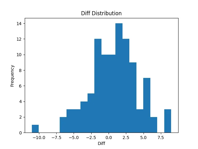
怀疑出现了过拟合